
Depending on which drone and camera you are using, the procedure in Photoscan/Metashape differs. Therefore this instruction is divided in different sections depending on the function of each sensor/drone. The Agisoft manual is well written and give you a deeper understanding about the workflow described below.
The guide goes through how you create an ortho photo and 3D point cloud from images taken with a drone.
Note to Metashape users who used Photoscan before: Some have noticed that they get a new grey theme and all icons are greyish instead of the colored ones present in Photoscan. In Metashape you can change the theme to the classic theme used in Photoscan: Tools – Preferences – General and look for “Theme:”. Select “classic” if you want the colored icons used in Photoscan.
For DJI Phantom 4 RTK we have made a video-tutorial on how to import and align the photos, see this link.
Content
- Import photos, location and accuracy
- Image quality
- Align photos
- Ground control points (GCP)
- Dense point-cloud and ortho photo
Import photos, location and accuracy
- If you have location accuracy stored in the EXIF-tag (e.g. Parrot Sequoia):
Go to “Tools”-menu –> “Preferences…” –> “Advanced”-tab and check “Load camera location accuracy from XMP meta data. - Add your photos in Photoscan: “Workflow” –> “Add photos…”.
- If non-geotagged photos (e.g. SmartPlanes):
Import the camera positions. The camera positions is imported by clicking “Import”-button in the “Reference”-window. Make sure that you choose the right columns for the files. If the file contains orientation data, check the “Load orientation” checkbox and choose the right columns. Choose the coordinate system that the camera positions are stored in. If you have accuracy estimations you can load them as well. - If your camera is rotated on the drone (e.g. SmartPlanes), you need to specify this under “Tools” –> “Camera Calibration…”. Under the tab “GPS/INS Offset”, specify “Yaw (deg)” to 90.
- Check the settings. Click the “Settings”-button in the “Reference”-window. If you’re using orientation data and haven’t imported orientation accuracy, we recommend that you increase the accuracy to 10-20 degrees if you’re not sure that you have much better accuracy than that.
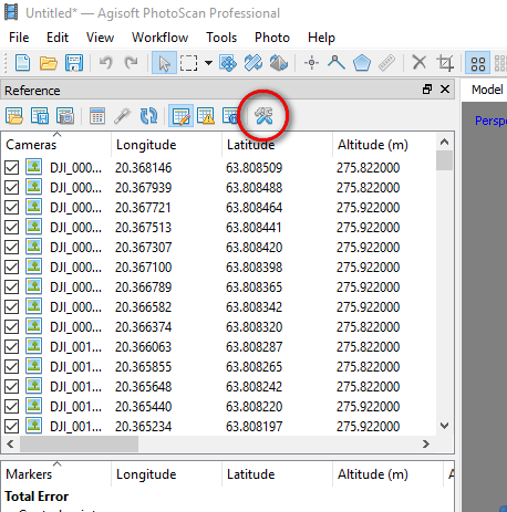
The “Settings”-button in the “Reference window”.
Image quality
- PhotoScan can automatically estimate image quality. Images
with quality value of less than 0.5 units are recommended to be disabled and thus excluded from the photogrammetric processing. - Image quality is estimated by right-clicking on a photo in the Reference-window, select “Estimate Image Quality…”, select “All cameras”.
- To display the estimated image quality of the photos, in the Photos pane change the view mode to “Details”. See screenshot below:
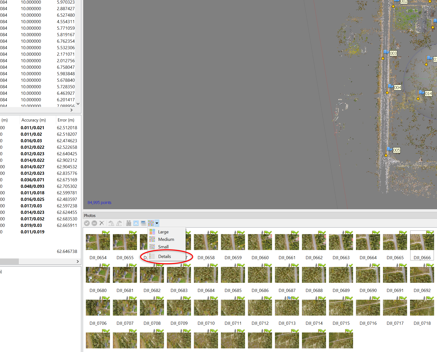
- You can now sort by the “Quality”-column. Select photos with lower quality than 0.5 and disable them.
Align photos
- Align your photos: “Workflow” –> “Align photos…”. Set “Accuracy” to “High” and “Pair preselection” to “Reference”. You can use “Highest” as well, but it will take longer time. Read in the manual what the accuracy levels mean. It can be necessary to adjust the “key point”- and “tie point”-limits to speed up the processing. The “Adaptive camera model fitting” will let Photoscan select which camera parameters that should be included in the adjustment based on their reliability estimate.
- After alignment has finished, go through your photos and uncheck and disable photos in turns of the photo-block. After you have done this, run “Optimize cameras…”. Check on: f, cx, cy, k1, k2, k3, p1, p2.
- Make a copy of your chunk before you proceed. This makes it possible to go back to your copy if something goes wrong in the following steps.
- Use the manual selection tools to remove obvious outlier points in the sparse point-cloud. Run “Optimize cameras…” (check on: f, cx, cy, k1, k2, k3, p1, p2).
- Use “Gradual selection…” under the “Model”-menu. It’s difficult to recommend a certain values to the filters, the best way is to iterate through these filters to achieve a point cloud with small errors. The values specified should be seen as recommendations and are dependent on the quality of your data. Use the following filters:
-
- Image count. Use this if you have data that should have more than two photos covering, for example open fields and clear-cuts. Then you can use image count = 2, but if you want the ground in forestry data, skip this one. Run “Optimize cameras…” with same parameters as before.
- Reconstruction uncertainty (geometry). Use the slider to adjust a suitable value to select points with high uncertainty. Recommended values: 50 to 25. Press OK and then delete the points by pressing Delete on the keyboard. Run “Optimize cameras…” with same parameters as before. Repeat this at least 2 times.
- Projection accuracy (pixel matching errors). Use the slider to adjust a suitable value to select points with high uncertainty. Recommended values: 10 to 8. Press OK and then delete the points by pressing Delete on the keyboard. Run “Optimize cameras…” with same parameters as before. Repeat this filter and optimization at least 2 times.
- “Optimize cameras…” with all parameters checked.
- If you have ground control points (GCP), import them now before you proceed to the next step (reprojection error). See below how you import GCP. Also align only using GCP.
- Reprojection error (pixel residual error). Use the slider to adjust a suitable value to select points with high uncertainty. Recommended values: 1 to 0.5. Press OK and then delete the points by pressing Delete on the keyboard. Run “Optimize cameras…” with all parameters checked. Repeat this at least 2 times.
-
Ground control points (GCP)
This step is only done if you have collected ground control points.
- If your ground control points (GCP) are in a different coordinate system to the images, you now need to transform your project to the same coordinate system as your GCP before you import them. This is done by clicking the “Convert” button in the “Reference”-window.
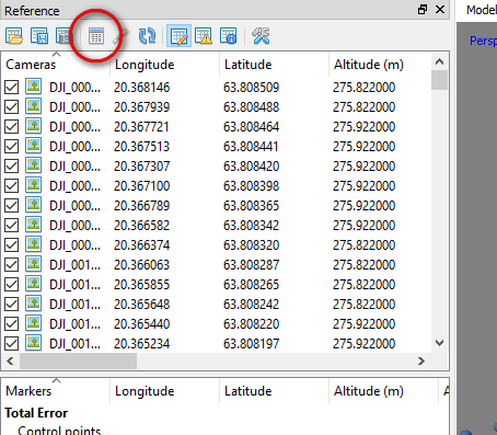
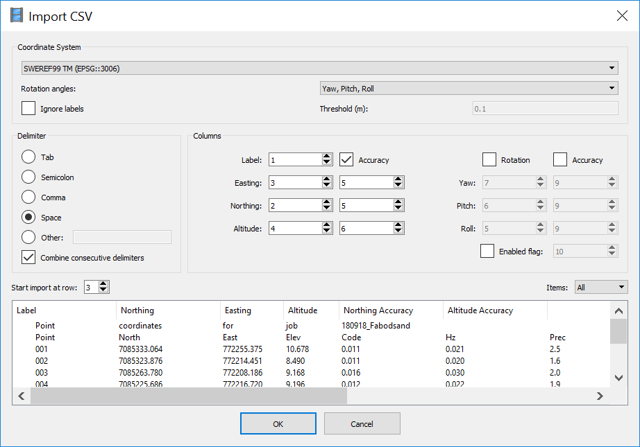
The button to click for coordinate system conversion. - Import GCP by clicking the “Import”-button in the “Reference”-window. The following settings should be done if you import GNSS-coordinates from the Trimble GeoXR (and exported the coordinates in Sweref99 TM RH2000):
- The accuracy for each GCP (or even photo) can be set in three different ways:
- 0.1 = 0.1 m accuracy in x, y and z.
- 0.1/0.5 = 0.1 m accuracy in x and y. 0.5 m accuracy in z.
- 0.1/0.2/0.5 = 0.1 m accuracy in x, 0.2 m accuracy in y and 0.5 m accuracy in z.
- Go through GCP by GCP and point them out in the photos. You can right-click on the GCP and choose “Filter photos by selection…”. You can switch between photos by using “Page Up” and “Page Down” keys. Place each marker in at least two photos. It will be easier as you go. Run “Optimize cameras…” time to time to improve the location of the non-placed markers.
- “Optimize cameras…”. If your GCPs are of high accuracy, then you should uncheck all photos before you click “Optimize cameras…”. Make sure that all GCP you want to use are checked and that they have appropriate settings of accuracy. For photos taken with a DJI-drone, the altitude is of bad quality and you should therefore always uncheck the photos before running “Optimize cameras…” and proceeding the processing (valid for DJI-drones up to year 2018 at least).
- When the above steps are done and the error in the GCP should be small (~5-20 cm if using RTK GNSS receiver).
Dense point-cloud and ortho photo
- Now you can either do a batch script doing the commands below or run them one by one.
- Build dense cloud. Use quality “high” (seldom use “Ultra high” because it takes long time and normally the photos don’t have that high quality. Read more in the manual). Set depth filtering to “mild”.
- Export dense cloud as las for example.
- Build mesh (normally from the sparse cloud).
- Smooth the mesh (Tools –> Mesh –> Smooth Mesh.
- Create ortho photo using the mesh from the sparse cloud.
- Export ortho photo as tif for example.