
This manual is specifically written for the instrument Trimble TX8. It is partly in Swedish at the moment, but will be translated to English if there is a need for that.
Content
Scanning
Single scan
Multiscan using 230 mm balls on the tripods
Georeferencing a multiscan
Postprocessing
Postprocessing a single scan
Postprocessing a multiscan using 230 mm balls on the tripods
Georeferencing scans
Generate points
Scanning
Single scan
This part has not been written yet.
Multiscan using 230 mm balls on the tripods
Exempel plockat från remningstorpsinventeirngen 2014. Denna har reviderats till en allmänt användbar version.
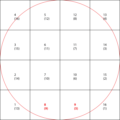
- Lokalisera delprovyta 1 (sydvästra hörnet. Inom parentes så anges namnet som användes vid fältinventeringen 2014).
- Ställ upp stativet. Det är bra om skannern är ganska högt upp, ca 1.5 meter ovan marken. Stampa ner stativfötterna ordentligt så det står statigt. Det är extremt viktigt att stativet inte rör sig när skannern sedan flyttas och bollar monteras istället.
- Nivellera plattan där skannern ska monteras. Markera stativet med A genom att hänga på A-bandet runt stativets topp.
- Montera skannern på stativet.
- Om referensträd skall användas för att referera fältmätningar mot laserskanningen så sätts dessa upp nu.
- Lokalisera delprovyta 8. Se till att det är fri sikt till skannern där stativet monteras. Detta är nu bakåtobjektet som sedan kommer att vara platsen för den 8:e skanningen.
- När du ställt upp stativet nivellerar du plattan. Markera detta stativ med bokstaven D (finns D-band som hängs runt stativets topp). Notera uppställningens bokstav i fältprotokollet.
- Montera en boll på stativet (230 mm). OBS: detta stativ med boll skall stå kvar fram t.o.m. den 7:e skanningen, stå kvar med skannern monterad under den 8:e skanningen och skall stå kvar med boll monterad under den 9:e skanningen.
- Lokalisera delprovyta 2. Sätt upp ett stativ så det är fri sikt till skannern (delprovyta 1). Det viktiga är att skannern ”ser” bollen på delprovyta 1.
- Nivellera plattan. Markera detta stativ med bokstaven B (finns B-band att hänga kring stativets topp).
- Montera en boll (230mm).
- Nu kan även stativet på delprovyta 3 monteras på samma sätts om för delprovyta 2, men är inget krav. Ett alternativ är att göra detta när skanningen pågår på delprovyta 1.
- Vrid skannern så att den startar ca 20 grader moturs nästa boll (delprovyta 2). Starta skanningen från delprovyta 1.
- Medan skanningen pågår monteras det fjärde stativet upp på delprovyta 3 (du kan gå till denna yta så snart skannern passerat din gångväg).
- Nivellera plattan. Markera stativet med bokstaven C (finns C-band att hänga runt stativets topp).
- Montera en boll på stativet (230 mm).
- Återgå till delprovyta 1 (ta med bollen från delprovyta 2) och verifiera att alla bollar och referensträd syns i skanningen.
- Fotografera mot nästa stativ samt mot föregående stativ. Fotograferingsriktningen anges av pilarna i fältprotokollet, likaså vilka bollar som syns från respektive skanningsuppställning.
- Stäng av skannern och flytta den till delprovyta 2. Starta upp skannern. Markörerna från referensträden på delprovytorna lämnas kvar i de flesta fall. Montera bollen på stativet på delprovyta 1.
- Vrid skannern så att den startar 20 grader moturs nästa boll (delprovyta 3). Skanna från delprovyta 2 och verifiera att alla bollar syns i skanningen.
- Ett stativ sätts upp på delprovyta 4 (flytta från delprovyta 1 och ta med tillhörande boll). Nivellera plattan. Montera bollen på stativet. Markera detta stativ med bokstaven A.
- Återgå till delprovyta 2 (ta med bollen från delprovyta 3) och verifiera att alla bollar och referensträd syns i skanningen. Stäng av skannern och flytta skannern till delprovyta 3. Starta upp skannern. Montera en boll på stativet på delprovyta 2. Vrid skannern så att den startar 20 grader moturs nästa boll (delprovyta 4). Starta skanningen från delprovyta 3 och kontrollera att alla bollar och referensträd syns i skanningen.
- Nu upprepas denna procedur. Principen är att det hela tiden måste finnas en boll framåt och en boll bakåt som är synliga för skanningen. Positionen för ett stativ får inte röras det minsta under den tid det är uppsatt eftersom det har tre funktioner: framåtobjekt, skannerplacering och bakåtobjekt. Bokstaven som hänger på stativet måste vara synliga i data. Används referensträd till fältdata måste de vara synliga i data och referensträdet mot norr måste kunna skiljas ut från de övriga. Om det direkt efter skanningen vid visuell kontroll av data visar sig att t.ex. en boll inte är synlig så görs denna skanning om efter det att sikten röjts genom att ta bort grenar (OBS: rör inte stativen). Proceduren upprepas fram till att delyta 6 är skannad.
- För delyta 7 används den boll som står kvar på delprovyta 8 från den första skanningen som framåtobjekt. Innan den 7:e skanningen genomförs flyttas stativet från delprovyta 5 till delprovyta 9 och används som extra framåtobjekt (om det är möjligt att röja sikten diagonalt mellan delyta 7 och 9).
- Stativet på delprovyta 9 lämnas kvar till dess skanning på yta 16 utförts.
- Före skanningen på delprovyta 10 flyttas stativ och boll från delprovyta 8 till delprovyta 11 och används som framåtobjekt. Sedan upprepas proceduren med att stega sig fram där bakåtobjektet blir stativet som användes i föregående skanning och framtåobjektet sätts ut genom att flytta stativet som var bakåtobjekt i föregående skanning. Detta utförs för resterande delprovytor. Vid den sista skanningen, delyta 16, är det viktigt att stativet vid delyta 9 syns (och dess boll).
Georeferencing a multiscan
This georeferencing guide assumes that you follow the workflow “Multiscan using 230 mm balls on the tripods“.
Montera GPS-antennen (Trimble Zephyr) på trefoten istället för en av de runda 230mm bollarna. Använd alltså även förlängningsadaptern som är 100mm.
In the GNSS receiver (Trimble GeoXR 6000):
- Set the antenna height to: -0.130 m when using the Topcon 100 mm distance (photo below). Note the minus sign.
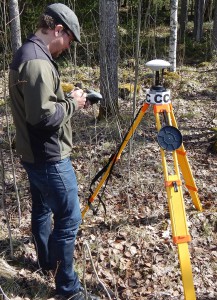
- Set the antenna measurement point to ”undersida av antennfästet”.
- Give the point a name that you can use in reference to the scanning station.
- Measure the point. If you get a fix solution, it’s enough if you measure for approximately 10 seconds. Without a fix solution, measure as long as possible before you store the point. More information about GNSS-measuring with the Trimble GeoXR 6000.

Postprocessing
Postprocessing is done in Trimble Realworks. This guide is written for Realworks version 10, but the procedure is probably the same in future versions. The software can be downloaded from: https://geospatial.trimble.com/products-and-solutions/trimble-realworks. The license dongel is stored in the scanners bag and has a green band. Plug in this dongel in a USB 2 port. Some times it doesn’t function i a USB 3 port.
Postprocessing a single scan
This part has not been written yet.
Postprocessing a multiscan using 230 mm balls on the tripods
- Copy the project from the scanners USB-stick to a local folder on your computer. It is recommended to copy the data to a folder named “RAW” or Delivery and then make a copy to a folder named “Processed”. You should now work on the folder “Processed”.
- Open Trimble Realworks.
- Open the “*.rwp” file connected to your project.
- Select the project in the workspace then go to the “Registration”-tab. Click “Auto-extract Targets”. Check “Spherical target”. Choose diameter “0.23 mm”. Uncheck “Black and White Flat Target” and also uncheck “Generate a Preview Scan”. Click OK.
- In the dialog box coming up, check the box “Compress TZF Scans”. Press OK.
- The computer will now automatically extract the targets (spheres). This takes quite some time.
After this has completed it is time to connect the single scannings with eachother. This is done by:
- The “Target-based registration” dialog box opens when the target extraction is finished.
- Click “Analyze”. The following dialog box opens:
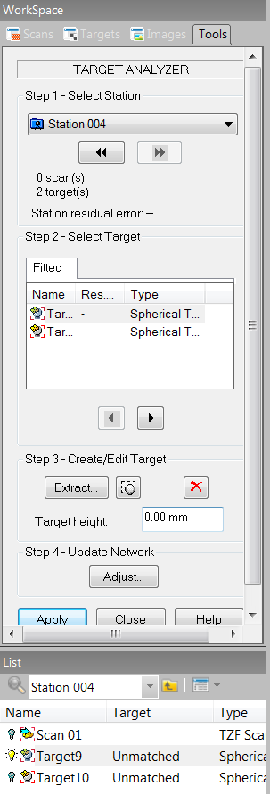
- Go through the targets station by station and check if the automatic extraction is correct. Click the target in the table “Fitted”. If the target is correct, rename it to a name connected to the scanning location, for example 1, 2, 3, 4… or A, B, C… Rename by selecting the current scanning location in the lower part of the workspace panel and then press F2.
- If a target is not correct. Highlight the target and click the red cross button to delete it. Delete both scanning and target.
- If a target is missing press Extract, click on the surface of the ball in the window named Scan. A fitting will be performed and the results are visualized in the window below. Scroll to zoom in and make sure that the pixels of the ball that you can observe match up to the fitted ball.
- When you are satisfied with the fit press create in the small window “Fitting” that have appeared. Name the station and the height from the ground if known. Close the small window “Target Creator”.
- When you have gone through all stations and targets, press “Apply”.
- You can now close the “Target-based registration” dialog box by clicking “Close”. Click “Yes” when asking “Do you want to apply all changes to database?”. Also click OK when asking “Do you really want to continue?”
- Rename the stations to have the same names as you gave the targets in step 3. This rename is done in the “Workspace” dialog box.
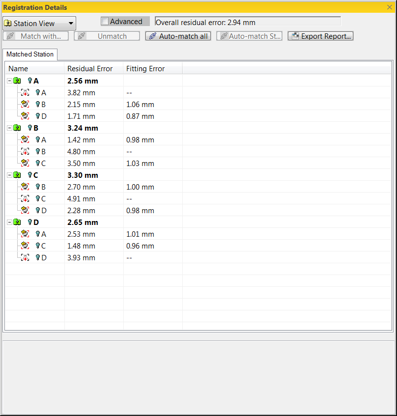
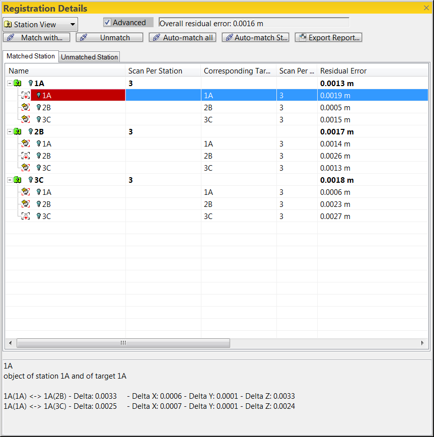
- Select the project in the workspace then go to the “Registration”, click “Name-based Network Adjustment” under “Survey Workflow”.
- You will now see a dialog box presenting the “Registration details”. The error is normally 1-3 mm (Residual Error).
- You can now group the four stations before you continue. This is done so you can proceed with georeferencing the points. If you don’t group the stations, they will move individually when georeferencing, but if you group, the will be locked in position between eachother and the whole group will move and fit to the coordinates you use for georeferencing. Click “New Group” in the workspace panel then drag each station inside the New group folder created in the workspace.
To create sampled scans (necessary if you want to export the point-cloud to las-format), do the following:
- Mark the “New group” in the Workspace dialog or the name you have given the new group.
- In the “Edit” tab, click “Create Sampled Scans” under the “Scan” group.
- If you want to extract all points, choose “Sampling by Step” and set “Step (in pixels)” to 1. This means you will extract every measurement. Press OK. The computer will now process all the scans and create a sampled scan for each station.
Note: If you follow the procedure for 16 scan locations you need to name the stations like: 1A, 2B, 3C, 4A, 5B, 6C, 7A, 8D, 9B, 10C, 11A, 12D, 13C, 14A, 15D, 16C. This is a way to remember which letter-tag that was hung on which tripod.
Georeferencing scans
- Open the project you want to georeference to world coordinates.
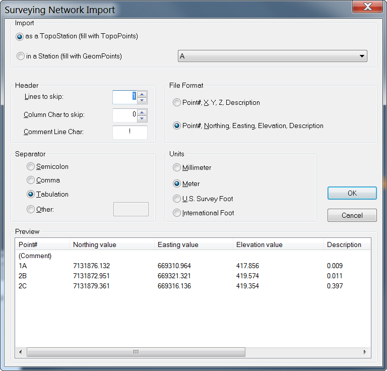
- Open the txt-file containing the coordinates of the scan stations or targets in the point cloud. The file is opened by clicking “Open” that can be found under the “Import/Export” section in the Home tab. Select the file and click “Open…”. Do the following settings:
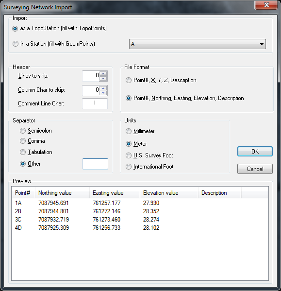
Under “Separator”, choose “Other:” and put a space in the box.
The file need to fulfill the following:
- File ending need to be .txt.
- Remove other information from the file except the following fields:
- Point #, Northing, Easting, Elevation, Description
- It is easier if you use tab as separator in the file. Notepad++ can be used to edit your textfile to fulfill the above conditions or you can use the R-script below that convert files from the Trimble GeoXR 6000 so the files are readable from Realworks:
[code lang=”r” wraplines=”TRUE”]
setwd("D:\\TLS\\GPS Points")
listOfFiles <- list.files(path=".", pattern=".txt")
dir.create("convertedFiles")
 
for(file in listOfFiles) {
 coord <- read.table(file=file, skip = 3, header=F)
 names(coord) <- c("Name", "North", "East", "Elev", "HzPrec", "VtPrec", "PDOP", "Sats")
 write.table(x = coord[ ,1:5], file = paste0("convertedFiles/", file), sep="\t", col.names = T, row.names = F, quote = F)
}
[/code]
Download the script. After the above code has been used to convert the files, you can do the following settings to import the points:
- Under the tab “Registration” click ”Target-Based Registration” under “Target-Based Registration”.
- When the tool opens, it will ask you if you want to automatically match the scan stations with the topo stations. You can answer “No” and do the following steps instead.
- Manual target matching:
- Click ”Check…”.
- Mark the first scan station with the scanner tripod icon. See example below:
Click “Match with…”. Choose the Topo point to match with scan station. - Continue to match the other scan stations with the topo points.
- When you have matched all stations with topo points, click “Adjust”.
- Press “Apply” in the toolbox.
- Press “Close” in the toolbox. The “Registration Details” window will now also close.
Generate points
To be able to work with the points within Realworks, you need to “sample” the scans. To achieve all points you do:
- Mark the stations you want to export in the list or mark the whole project in the Workspace.
- Click the “Home”-tab. Click “Create Sampled Scans” under “Extraction”.
- Select “Sampling by step”. Choose 1 pixel if you want all points. Press OK.
Report
Create the following reports for each scanning project:
Report of targets
- Markera projektet i Workspace-listan.
- Home – Export – Export Object Properties…
- Namnge filen till namnet på skanningsuppställningen.
- Under Option, kryssa i ”Project of selection”.
- Spara filen.
Rapport på registrering
- Markera projektet i Workspace-listan.
- Registration – Registration Report (Target-Based).
- Spara filen.
Position på skanningsuppställningar
Detta ger dig en position på respektive skanningsuppställning.
- Markera projektet i Workspace-listan.
- Registration – RMX – Export Station Registration Parameters to RMX Files…
- Välj en mapp.
- Detta kommer ge dig en mapp med RMX-filer där koorinat för centrum av varje skanningsuppställning går att utläsa.
Storage / backup
Nedan följer ett exempel på hur ett projekt kan dokumenteras och lagras för arkivering.
Bilder – Här lagras foton som togs i samband med skanningen. Sorterad ytvis.
Film – Filmer som skapats för att demonstrera data.
LAS_diverseExporter – Diverse exporter som kan användas för att demonstera data.
LAZ_full – LAZ-filer av samtliga ytor. Varje fil innehåller samtliga punkter och är komprimerade med laz. Program för att packa upp ligger i katalogen.
Processed_data – Ett Realworks projekt för varje yta. Varje skanningsuppställning består av en tzf-fil som är komprimerad. Hela ytor är sammansatta via named based registration. Varje projekt innehåller också en sampled skan för varje delyta som inte är reducerad (1px sampling).
Rapport – Innehåller rapport som beskriver hur skanningen utförts och processerats, inskannade fältprotokoll och en excel-fil med sammanställning av skannade ytor, koordinater. Innehåller även en undermapp (Projektrapporter) med en rapport för respektive yta med egenskaper samt registeringsrapport som exporterats ur Realworks.
RAW_data – RAW-data som det såg ut när det kopierades från skannern. Här finns kan även skanningsuppställningar finnas med som skannats dubbelt pga att bollen på stativen inte syntest vid första skanningen. Dessa uppställningar har raderats i Processed_data.
RMX – En fil för varje skanningsuppställning med koordinater och rotation (lokalt koordinatsystem).